Curve Fitting in PyARPES#
Why curve fit#
Curve fitting is an extremely important technique in angle resolved-photoemission because it provides a coherent way of dealing with sometimes noisy data, allows for simple treatment of backgrounds, avoids painful questions of interpretation inherent with some techniques, and grants access to the rich information ARPES provides of the single particle spectral function.
Simple curve fitting#
PyARPES uses lmfit in order to provide a user friendly,
compositional API for curve fitting. This allows users to define more
complicated models using operators like + and *, but also makes
the process of curve fitting transparent and simple.
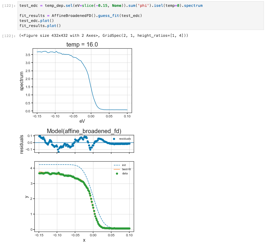
Here we will prepare an EDC with a step edge, and fit it with a linear
density of states multiplied by the Fermi distribution and convolved with
Gaussian instrumental broadening (AffineBroadenedFD). In general in
PyARPES, we use extensions of the models available in lmfit, which
provides an xarray compatible and unitful fitting function
guess_fit. This has more or less the same call signature as fit
except that we do not need to pass the X and Y data separately, the X
data is provided by the dataset coordinates.
A simple curve fitting example#
The results of a fit should also provide a useful summary table if you print them in Jupyter.
Jupyter will print tables summarizing curve fitting results#
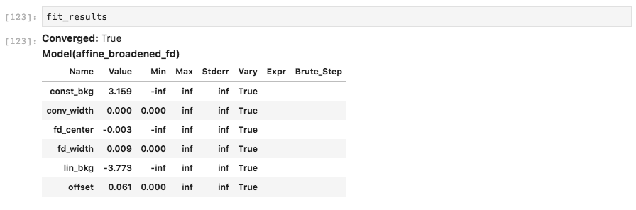
Using the params= keyword you can provide initial guess with
value, enforce a max or min, and request that a parameter be
allowed to vary or not. In this case, we will force a fit with the
step edge at 10 millivolts, obtaining a substantially worse result.
An example holding parameters constant#
A number of models already exist including lineshapes, backgrounds, and step edges. All of these can also be easily composed to handle several lineshapes, or convolution with instrumental resolution:
arpes.fits.fit_models.GaussianModelarpes.fits.fit_models.VoigtModelarpes.fits.fit_models.LorentzianModelarpes.fits.fit_models.AffineBackgroundModelarpes.fits.fit_models.GStepBModel- for a Gaussian convolved low temperature step edgearpes.fits.fit_models.ExponentialDecayModelarpes.fits.fit_models.ConstantModelarpes.fits.fit_models.LinearModelarpes.fits.fit_models.FermiDiracModelarpes.analysis.gap.AffineBroadenedFD- for a linear density of states with Gaussian convolved Fermi edge
Adding additional models is very easy, especially if they are already
part of the large library of models in lmfit. If you are interested,
have a look at the definitions in arpes.fits.fit_models.
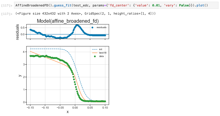
Broadcasting fits#
While curve fitting a single EDC or MDC is useful, often we will want to repeat an analysis across some experimental parameter or variable, such as the binding energy to track a dispersion, or across temperature to understand a phase transition.
By the previous version of PyARPES, a tool broadcast_model that allows
for automatic and compositional curve fitting across one or more axes of a Dataset or
DataArray is provided. While it was nicely convenient, but it might be somehow
complicated and difficult to maintain. At present, xarray has curvefit metohd.
Unfortunately, this method is not so suitable to handle lmfit model, which is more flexible, and used in PyARPES.
Fortunatelely, xarray-lmfit is made with reference of xr.DataArray/Dataset.curvefit.
While xarray-lmfit does not work in parallel for xr.DataArray,
the current computational speed sufficiently high. This is not the serious problem.
Thus we have decided to drop broadcast_model and use xarray-lmfit internally.
By using S.modelfit method, the multidimentional fitting can be easily performed.
A broadcasted curve fitting example#
The resultant of the fitting is stored as the xr.Dataset. As same as the previous version,
The .F extension to xarray in order to access the fitting results.
This is necessary because the result of a fit is a
Dataset containing the full data, including the experimental data. The
results attribute is itself a DataArray whose values are the full
results of the fit, rather than any single of the values.
Because of the rich information provided by a S.modelfit (xarray-lmfit), PyARPES also
has facilities for interacting with the results of an array of fit
results more simply, furnished by the .F attribute.
The .F attribute#
You can get all the parameter names with .parameter_names.
Getting fit values#
Using the .F attribute we can obtain the values for (p) as well
as the fit error of (s) any fit parameters we like.
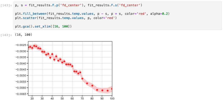
The p and s getters#
Quickly plotting a fit#
We can also quickly plot a fit result with plot_param. This is
sometimes useful for immediately plotting a fit result onto data or
another plot sequence.
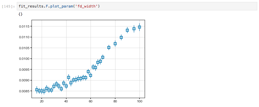
The plot_param function#
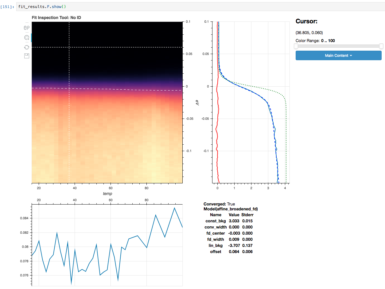
Examining fit quality interactively#
Fit results can also be explored interactively with .F.show(),
similar to .S.show for spectra.
The plot_param function#
Fitting complex lineshapes semi-interactively#
In addition to looking at the results of fits interactively, you can
also lay down lineshapes for one or more dispersive bands with
.S.show_band_tool(). Follow roughly the information provided for
masking to get started. The “Center Constraint” value dictates how much
the lineshape is allowed to vary from the approximate location you lay
down.
Using the “Mode” setting, you can choose whether EDCs or MDCs will be
fit. Should more than one band (or the same band more than once) cross a
given EDC or MDC during the fit, the appropriate number and location of
lineshapes will be used. As a result of one band crossing an EDC or MDC
more than once, the fit parameters will be postfixed with _{number}
to indicate the index of the crossing.
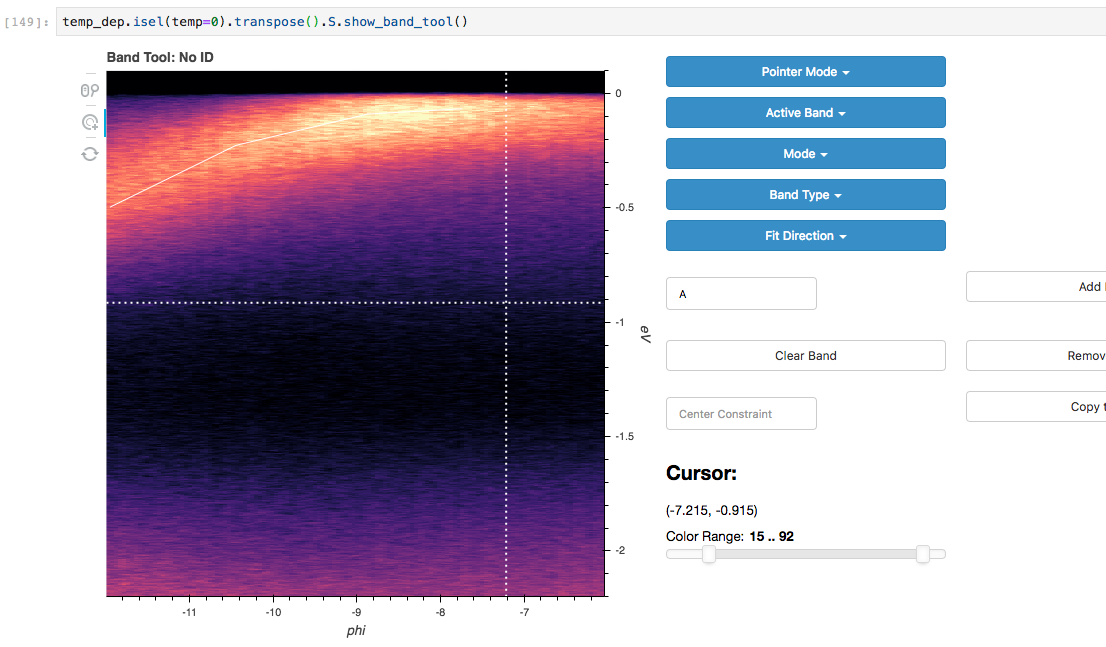
Band tool#