Curve Fitting in PyARPES#
Why curve fit#
Curve fitting is an extremely important technique in angle resolved-photoemission because it provides a coherent way of dealing with noisy data, it allows for simple treatment of backgrounds, it avoids painful questions of interpretation inherent with some techniques, and it grants access to the rich information ARPES provides of the single particle spectral function.
Simple curve fitting#
PyARPES uses lmfit in order to provide a user friendly, compositional API for curve fitting. This allows users to define more complicated models using operators like + and *, but also makes the process of curve fitting transparent and simple.
Here we will prepare an EDC with a step edge, and fit it with a linear density of states multiplied by the Fermi distribution and convolved with Gaussian instrumental broadening (AffineBroadenedFD). From Ver. 5.0 of PyARPES, we use xarray-lmfit package, which provides an xarray compatible and unitful fitting function. By this change, the coordinate must be specified explicitly. While one may feel that it many be not elegant, we believe that it follows Zen of python “Explicit is better than
implicit”. And reagardless the dimension of the data, we can take the same procedure for fitting. And if you experienced lmfit, the operation process quite easy to understand. Use S.modelfit instead of fit function as follows.
[1]:
import arpes

# first let's prepare some data to curve fit
from arpes.io import example_data

test_edc = (
    example_data.temperature_dependence.spectrum.sel(eV=slice(-0.15, None))
    .sum("phi")
    .isel(temperature=0)
)

test_edc.plot()
Activating auto-logging. Current session state plus future input saved.
Filename       : logs/unnamed_2026-03-24_23-28-38.log
Mode           : backup
Output logging : False
Raw input log  : False
Timestamping   : False
State          : active
[1]:
[<matplotlib.lines.Line2D at 0x7071604637a0>]
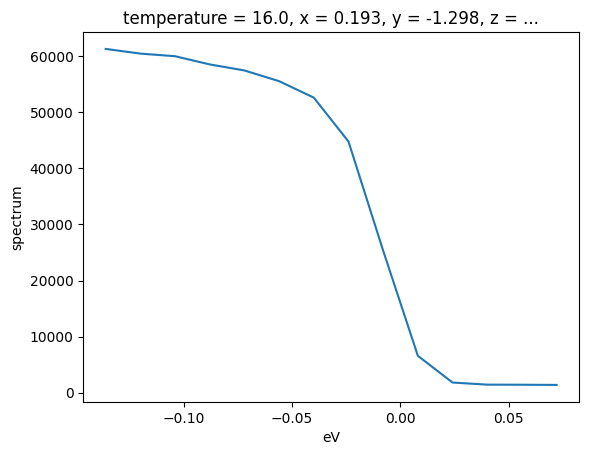
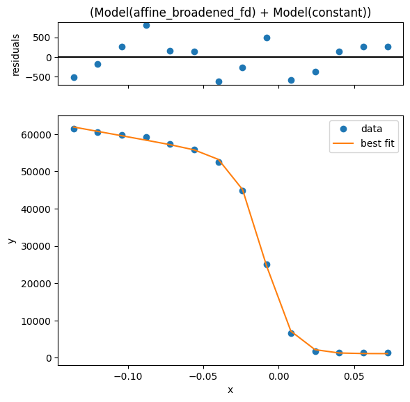
Now, let’s fit this data with a broadened edge.
[2]:
from lmfit.models import ConstantModel
from arpes.fits.fit_models import AffineBroadenedFD

affine_model = AffineBroadenedFD()
params = affine_model.guess(test_edc, test_edc.coords["eV"])
model = affine_model + ConstantModel()
result = test_edc.S.modelfit("eV", model, params=params)


result.modelfit_results.item().plot()  # plot the fit, residual, etc
result.modelfit_results.item()  # print parameters and info
[2]:
Fit Result
Model: (Model(affine_broadened_fd) + Model(constant))
| fitting method | leastsq |
| # function evals | 59 |
| # data points | 14 |
| # variables | 6 |
| chi-square | 2315116.65 |
| reduced chi-square | 289389.582 |
| Akaike info crit. | 180.222786 |
| Bayesian info crit. | 184.057130 |
| R-squared | 0.99974919 |
| name | value | initial value | min | max | vary |
|---|---|---|---|---|---|
| center | -0.00921419 | -0.03189873695373535 | -inf | inf | True |
| width | 0.00877083 | 0.020800971984863283 | 0.00000000 | inf | True |
| sigma | 6.4200e-04 | 0.020800971984863283 | 0.00000000 | inf | True |
| const_bkg | 51191.6673 | 59886.28125 | -inf | inf | True |
| lin_slope | -75038.6829 | 0.0 | -inf | inf | True |
| c | 1120.78461 | 0.0 | -inf | inf | True |
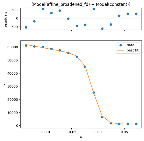
Empirically, we have a very good fit. One thing it is good to know about resolution convolved edges is that there are two width parameters: width and sigma. These are the intrinsic edge width caused by thermally excited carriers in the Fermi-Dirac distribution and a broadening which affects the entire spectrum due to instrumental effects, respectively.
Because these can have nearly degenerate effects if you have only a single edge with no peak, you may want to set one parameter or another to an appropriate value based on known experimental conditions.
From your analyzer settings and photon linewidth, you may know your resolution broadening, while from the temperature you may know the intrinsic edge width.
Before moving on, the tabular representations of parameters above was produced by letting the cell output be result.
Influencing the fit by setting parameters#
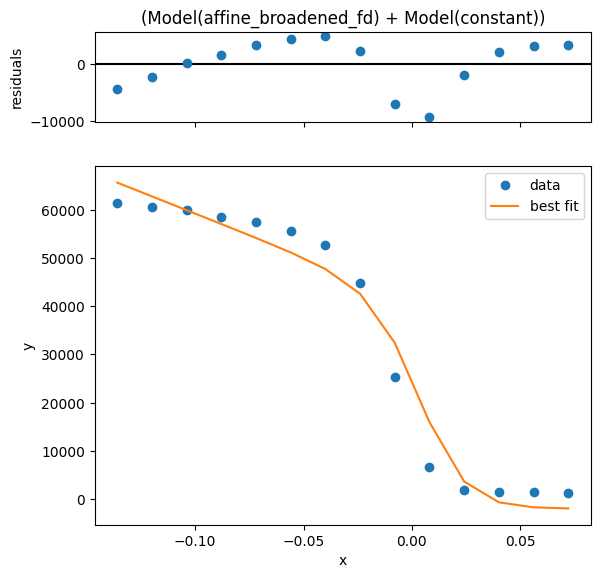
Using the params= keyword you can provide initial guess with value, enforce a max or min, and request that a parameter be allowed to vary or not. In this case, we will force a fit with the step edge at 10 millivolts, obtaining a substantially worse result.
Let’s fit again but request that the step edge must be found at positive five millivolts.
[3]:
params["center"].value = 0.005
params["center"].vary = False
guess_fit_result = test_edc.S.modelfit("eV", model, params=params).modelfit_results.item().plot()
Overview of some models#
A number of models are already defined in lmfit including lineshapes, backgrounds, and step edges. All of these can also be easily composed to handle several lineshapes, or convolution with instrumental resolution:
The below is a list defined in PyARPES
arpes.fits.fit_models.AffineBackgroundModelarpes.fits.fit_models.GStepBModel- for a Gaussian convolved low temperature step edgearpes.fits.fit_models.ExponentialDecayModelarpes.fits.fit_models.FermiDiracModelarpes.analysis.gap.AffineBroadenedFD- for a linear density of states with Gaussian convolved Fermi edge
Adding additional models is very easy, especially if they are already part of the large library of models in lmfit. If you are interested, have a look at the definitions in arpes.fits.fit_models.
Also, remember that you can combine models using standard math operators.
Broadcasting fits#
While curve fitting a single EDC or MDC is useful, often we will want to repeat an analysis across some experimental parameter or variable, such as the binding energy to track a dispersion, or across temperature to understand a phase transition.
Due to the xarray-lmfit package, fitting to the 2D data by the same way. As same as the 1D data fitting, you can use lhe params= keyword to enforce constraints or specify initial guesses for the fitting parameters. Here we demonstrate performing the fitting procedure as a function of the sample temperature, and then plot the step edge location onto the data.
Note to the previous users: broadcast_model is removed. If you really keep to use this, go back to Ver. 4 series.
[4]:
import matplotlib.pyplot as plt

temp_edcs = example_data.temperature_dependence.sel(eV=slice(-0.15, None)).sum("phi").spectrum

params["center"].vary = True
params["sigma"].value = 0.0
params["sigma"].vary = False

fit_results = temp_edcs.S.modelfit("eV", model, params=params)

temp_edcs.T.plot()
plt.scatter(
    fit_results.modelfit_results.F.p("center").coords["temperature"],
    fit_results.modelfit_results.F.p("center").values,
    color="red",
)
[4]:
<matplotlib.collections.PathCollection at 0x70715e1fa5a0>
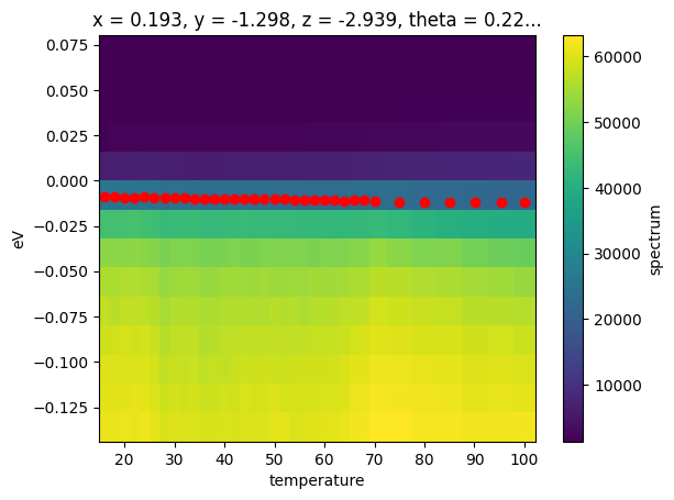
In the above, we also used the .F extension to xarray in order to get the concrete values of the center fit parameter as an array. This is necessary because the result of a S.modelfit is a Dataset containing the full data including the original experimental one. The modelfit_results DataArray is itself a DataArray whose values are the full results of the fit, rather than any single of the values.
Note for the previous version user: After using xarray_lmfit package, modelfit_results plays the same role of the results attribute.
Because of the rich information provided, PyARPES also has facilities for interacting with the results of an array of fit results more simply, furnished by the .F attribute.
The .F attribute#
You can get all the parameter names with .parameter_names.
Getting fit values#
Using the .F attribute we can obtain tjhe values for (p) as well as the fit error of (s) any fit parameters we like.
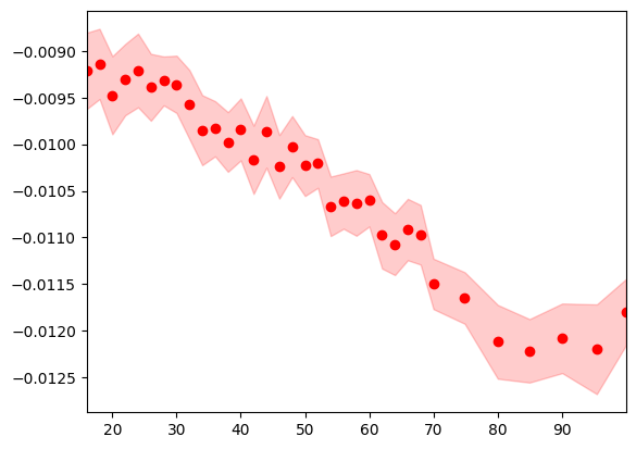
[5]:
p, s = fit_results.modelfit_results.F.p("center"), fit_results.modelfit_results.F.s("center")

fig, ax = plt.subplots()
ax.fill_between(fit_results.temperature.values, p - s, p + s, color="red", alpha=0.2)
ax.scatter(fit_results.temperature.values, p, color="red")

ax.set_xlim(fit_results.temperature.values[[0, -1]])
[5]:
(16.0, 99.98)
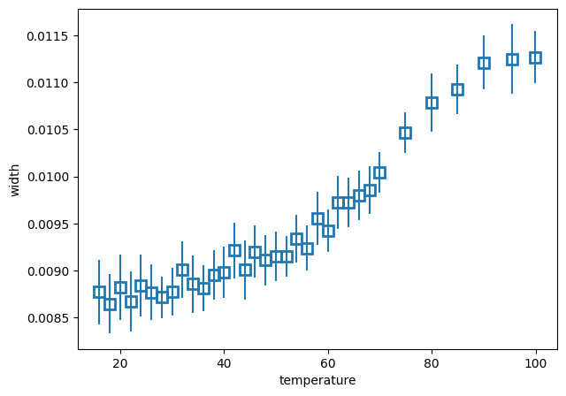
Quickly plotting a fit#
We can also quickly plot a fit result with plot_param. This is sometimes useful for immediately plotting a fit result onto data or another plot sequence.
[6]:
from arpes.config import use_tex

use_tex()
fit_results.modelfit_results.F.plot_param("width")
[6]:
<Axes: xlabel='temperature', ylabel='width'>
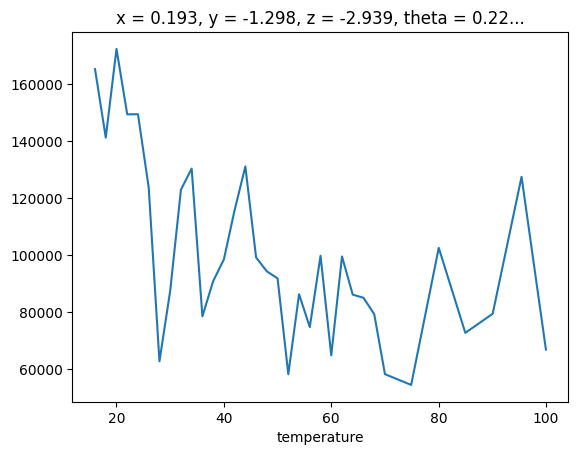
Introspecting fit quality#
Typically, you want to see the worst fits, so that you have some idea of how to refine them.
[7]:
worst_fit = fit_results.modelfit_results.F.worst_fits()[0].item()  # <- Not property work after V5.0
worst_fit_ = worst_fit.plot()
Based on this we can say that all the fits are very good. However, we may want to see how much variation there is in quality.
We can look at the .F.mean_square_error method for this information.
[8]:
fit_results.modelfit_results.F.mean_square_error().plot()
[8]:
[<matplotlib.lines.Line2D at 0x70715bd8d970>]
Interactively inspecting fits#
There’s no substitute for inspecting fits by eye. PyARPES has holoviews based interactive fit inspection tools. This is very much like profile_view which we have already seen with the addition that the marginal shows the curve fitting information for a broadcast fit.
Additionally, you can use the tool to copy any given marginal’s parameters to a hint dictionary which you can pass into the curve fit for refinement.
[9]:
from arpes.plotting import fit_inspection

# note, you can also run fit_results.F.show()
fit_inspection(fit_results, use_quadmesh=True)
[9]: