Data Abstraction#
The core data primitive in PyARPES is the xarray.DataArray. However, adding additional scientific functionality is needed since xarray provides only very general functionality. The approach that we take is described in some detail in the xarray documentation at extending xarray, which allows putting additional functionality on all arrays and datasets on particular, registered attributes.
In PyARPES we use a few of these:
.Sattribute: functionality associated with spectra (physics here).Gattribute: general abstract functionality that could reasonably be a part of xarray core.Fattribute: functionality associated with curve fitting
Caveat: In general these accessors can and do behave slightly differently between datasets and arrays, depending on what makes contextual sense.
This section will describe just some of the functionality provided by the .S attribute, while the following section will describe some of the functionality on .G and the section on curve fitting describes much of what is available through .F.
Much more can be learned about them by viewing the definitions in arpes.xarray_extensions.
Data selection#
select_around and select_around_data#
As an alternative to interpolating, you can integrate in a small rectangular or ellipsoidal region around a point using .S.select_around. You can also do this for a sequence of points using .S.select_around_data.
These functions can be run in either summing or averaging mode using either mode='sum' or mode='mean' respectively. Using the radius parameter you can specify the integration radius in pixels (int) or in unitful (float) values for all (pass a single value) or for specific (dict) axes.
select_around_data operates in the same way, except that instead of passing a single point, select_around_data expects a dictionary or Dataset mapping axis names to iterable collections of coordinates.
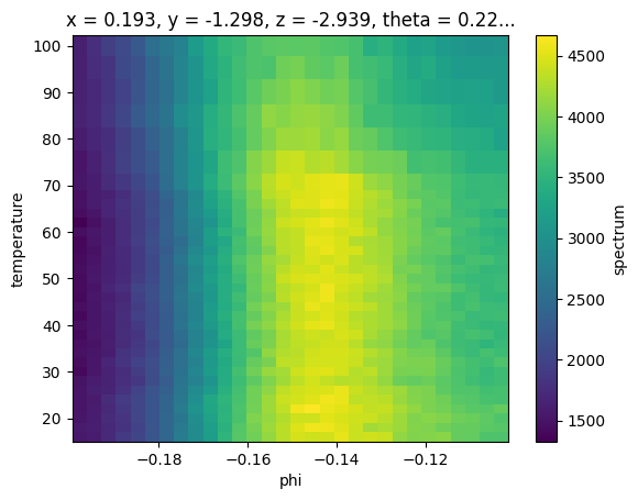
As a concrete example, let’s consider the example_data.temperature_dependence dataset with axes (eV, phi, T) consisting of cuts at different temperatures. Suppose we wish to obtain EDCs at the Fermi momentum for each value of the temperature.
First we will load the data, and combine datasets to get a full temperature dependence.
[1]:
import arpes
from arpes.io import example_data
from matplotlib import pyplot as plt

temp_dep = example_data.temperature_dependence
near_ef = temp_dep.sel(eV=slice(-0.05, 0.05), phi=slice(-0.2, None)).sum("eV").spectrum
near_ef.S.plot()
Activating auto-logging. Current session state plus future input saved.
Filename       : logs/unnamed_2026-03-24_23-28-50.log
Mode           : backup
Output logging : False
Raw input log  : False
Timestamping   : False
State          : active
Finding \(\phi_F\)/\(k_F\)#
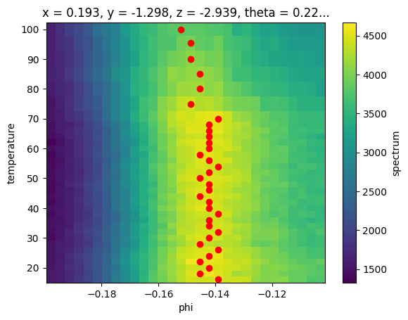
Now, we want to find the location of the peak in each slice of temperature so we know where to take EDCs.
We will do this in two ways:
Taking the argmax across
phiCurve fitting MDCs
Argmax#
[2]:
argmax_indices = near_ef.argmax(dim="phi")
argmax_phis = near_ef.phi[argmax_indices]

fig, ax = plt.subplots()
near_ef.S.plot(ax=ax)
# ax.scatter(*argmax_phis.G.to_arrays()[::-1], color="red")  # G.to_arrays is deprecated.
ax.scatter(argmax_phis.coords["phi"].values, argmax_phis.coords["temperature"].values, color="red")
fig
[2]:
Curve fitting#
This might be okay depending on what we are doing, but curve fitting is also straightforward and gives better results.
[3]:
from lmfit.models import LinearModel, LorentzianModel

# Fit with two components, a linear background and a Lorentzian peak
model = LinearModel(prefix="a_") + LorentzianModel(prefix="b_")
lorents_params = LorentzianModel(prefix="b_").guess(
    near_ef.sel(temperature=20, method="nearest").values, near_ef.coords["phi"].values
)
phis = near_ef.S.modelfit("phi", model, params=lorents_params)

phis
[3]:
<xarray.Dataset> Size: 30kB
Dimensions:                (temperature: 34, param: 5, cov_i: 5, cov_j: 5,
                            fit_stat: 9, phi: 30)
Coordinates: (12/15)
  * temperature            (temperature) float64 272B 16.0 18.0 ... 95.44 99.98
  * param                  (param) <U11 220B 'a_slope' ... 'b_sigma'
  * cov_i                  (cov_i) <U11 220B 'a_slope' ... 'b_sigma'
  * cov_j                  (cov_j) <U11 220B 'a_slope' ... 'b_sigma'
  * fit_stat               (fit_stat) <U8 288B 'nfev' 'nvarys' ... 'rsquared'
  * phi                    (phi) float64 240B -0.1978 -0.1946 ... -0.1063 -0.103
    ...                     ...
    theta                  float64 8B 0.2273
    beta                   float64 8B 0.0
    chi                    float64 8B -0.2618
    hv                     float64 8B 55.4
    alpha                  float64 8B 1.571
    psi                    int32 4B 0
Data variables:
    modelfit_results       (temperature) object 272B <lmfit.model.ModelResult...
    modelfit_coefficients  (temperature, param) float64 1kB 2.299e+04 ... 0.0...
    modelfit_stderr        (temperature, param) float64 1kB 877.6 ... 0.001892
    modelfit_covariance    (temperature, cov_i, cov_j) float64 7kB 7.703e+05 ...
    modelfit_stats         (temperature, fit_stat) float64 2kB 50.0 ... 0.9954
    modelfit_data          (temperature, phi) float64 8kB 1.535e+03 ... 3.066...
modelfit_best_fit (temperature, phi) float64 8kB 1.409e+03 ... 3.037...There’s a lot here to digest, the result of our curve fit also produced a xr.Dataset! This is because it bundles the fitting results (a 1D array of the fitting instances), the original data, and the residual together.
We will see more about all of this in the curve fitting section to follow. For now, let’s just get the peak centers.
[4]:
fig, ax = plt.subplots()
# ax.scatter(*phis.results.F.p("b_center").G.to_arrays()[::-1], color="red")
near_ef.S.plot(ax=ax)
ax.scatter(
    phis.modelfit_results.F.p("b_center").values,
    phis.modelfit_results.F.p("b_center").coords["temperature"].values,
    color="red",
)
fig
[4]:

This looks a lot cleaner, although our peaks may be biased too far to negative phi due to the asymmetric background.
Here, note that prefix “b_” is added to the parameter “center” of the LorentzianModel. (“b” means the “second” fitting model in this procedure)
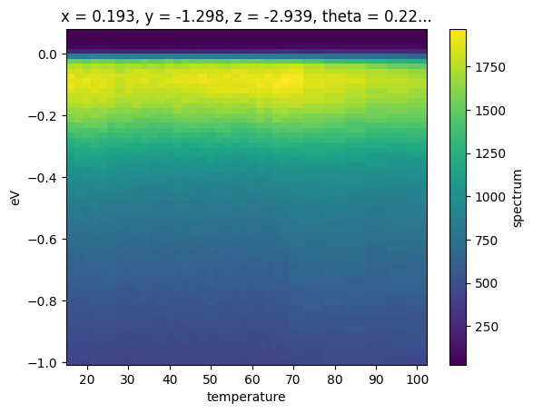
With the values of the Fermi momentum (in angle space) now in hand, we can select EDCs at the appropriate momentum for each value of the temperature.
Let’s average in a 10 mrad window.
[5]:
# take the Lorentzian (component `b`) center parameter
phi_values = phis.modelfit_results.F.p("b_center")
fig, ax = plt.subplots()
ax = temp_dep.spectrum.S.select_around_data(
    {"phi": phi_values}, mode="mean", radius={"phi": 0.005}
).S.plot(ax=ax)
fig
[5]:
Exercises#
Change the
phirange of the selection to see how the fit responds. Can we deal with the asymmetric background this way?Inspect the first fit with
phis.results[0].item(). What can you tell about the fit?Select a region of the temperature dependent data away from the band. Perform a broadcast fit for the Fermi edge using
arpes.fits.fit_models.AffineBroadenedFD. Does the edge position shift at all? Does the edge width change at all? Look at the previous exercise to determine which parameters to look at.