Intermediate Data Manipulation

import matplotlib.pyplot as plt

import arpes
from arpes.io import example_data

f = example_data.cut

Activating auto-logging. Current session state plus future input saved.
Filename       : logs/unnamed_2026-03-24_23-29-10.log
Mode           : backup
Output logging : False
Raw input log  : False
Timestamping   : False
State          : active

Data rebinning

Frequently it makes sense to integrate in a small region around a single value of interest, or to reduce the size of a dataset uniformly along a particular axis of set of axes. Rebinning the data can be used to accomplish both:

from arpes.analysis.general import rebin

fig, ax = plt.subplots()

ax = rebin(f, phi=15).S.plot(ax=ax)

Arguments passed into rebin after the first will be matched to dimensions on the input data. In this case, we have requested that every 12 pixels in ‘phi’ be rebinned into a single pixel. This reduces the size from 240x240 to 240x20. One can also rebin along multiple axes, with different granularities, simultaneously.

Getting help

Jupyter makes it convenient to get information about language and library functions, you just put a question mark after the function name. We can do this to see what information PyARPES has annotated onto rebin in the code

?rebin

Normalizing along an axis

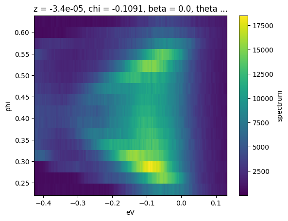
Another common pattern is to normalize data along an axis, so that the total intensity in each frame or slice is equal. This is relatively common in laser-ARPES in combination or as a comparison to normalization by the photocurrent. Another use case is in examining the role of matrix elements in photoemission, or in preparing data to be scaled and plotted on the same axes. normalize_dim can be used to normalize along one (second argument str) or several (second argument [str]) axes:

from arpes.preparation import normalize_dim

fig, ax = plt.subplots()
# make slices equal intensity at every energy
ax = normalize_dim(f.spectrum, "eV").plot(ax=ax)

In this case normalizing along the binding energy axis makes the surface state dispersion from room temperature photoemission off \(\text{Bi}_2\text{Se}_3\) for a substantial energy range above the chemical potential.

Broadcasting

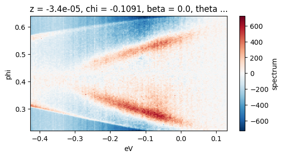
One simple way to achieve background subtraction is to take the mean of the data along a direction known to be a symmetry point, or a point away from dispersive intensity. In general all math operations on xarray instances broadcast just as you might expect if you have worked with numpy.

In particular, this means that if we create an EDC and subtract it from a spectrum, the EDC will be subtracted from every EDC of the spectrum, uniformly across other axes. We can use this to perform a simple subtraction, here of the EDC at the Gamma point of a \(\text{Bi}_2\text{Se}_3\) cut.

fig, ax = plt.subplots()

ax = (f - f.sel(phi=slice(0.42, 0.44)).mean("phi")).S.plot(ax=ax)
fig.set_figheight(3)

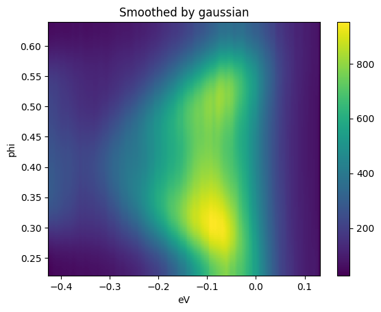
Smoothing

There are a number of smoothing facilities included, that are essentially wrappers around those provided in scipy.ndimage and scipy.signal. More details and other kernels can be found in arpes.analysis.filters. Here, we smooth a cut, only along the angular axis, against a Gaussian kernel with a width of 40 mrads.

from arpes.analysis.filters import gaussian_filter_arr

fit, ax = plt.subplots()
gaussian_filter_arr(f.spectrum, sigma={"phi": 0.04}).S.plot(ax=ax)
ax.set_title("Smoothed by gaussian")
fig.set_figheight(3)
fig.tight_layout()

Derivatives and Minimum Gradient/Maximum curvature

Facilities for taking derivatives along specified axes can be found in arpes.analysis.derivative. Additionally, the minimum gradient method and maximum curvature is supported.

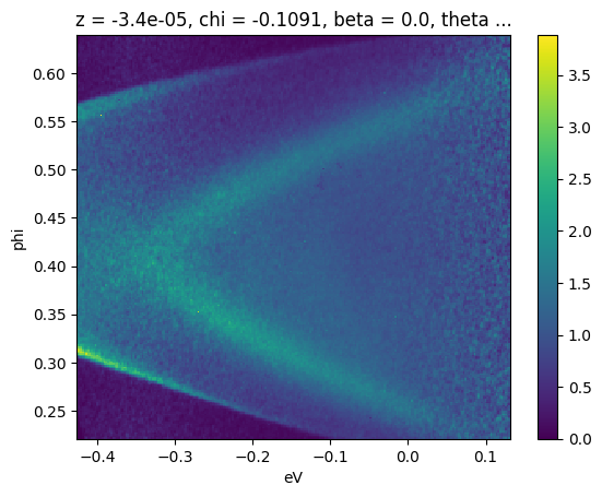
Here we illustrate the use of the minimum gradient after smoothing due to small statistics on sample data:

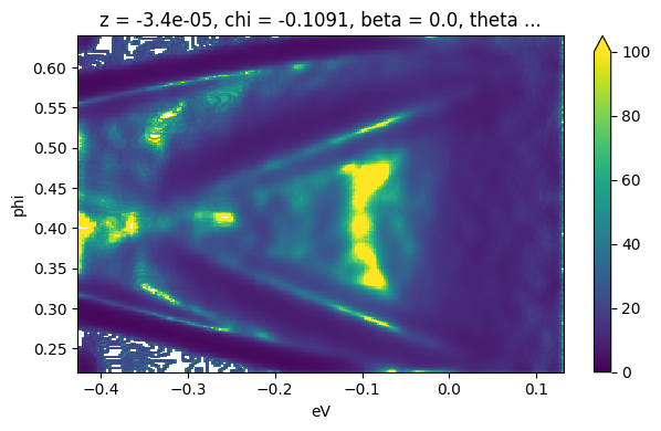
from arpes.analysis.derivative import minimum_gradient

fig, ax = plt.subplots()
ax = minimum_gradient(gaussian_filter_arr(f.spectrum, sigma={"phi": 0.01, "eV": 0.01})).plot(
    vmin=0,
    vmax=100,
)

fig.set_figheight(4)
fig.tight_layout()

This way shows the same result but is convenient in some case.

import functools

fig, ax = plt.subplots()

smooth_fn = functools.partial(gaussian_filter_arr, sigma={"phi": 0.01, "eV": 0.01})
ax = minimum_gradient(f.spectrum, smooth_fn=smooth_fn).plot(vmin=0, vmax=100, ax=ax)

fig.set_figheight(4)
fig.tight_layout()

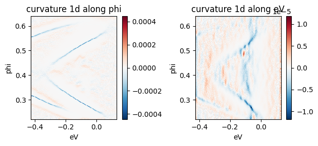
The Maximum curvature method has two types: 1D and 2D.

These two below are the example of 1D maximum curvature

from arpes.analysis.derivative import curvature1d, curvature2d

fig, ax = plt.subplots(1, 2)
curvature1d(
    gaussian_filter_arr(f.spectrum, sigma={"phi": 0.01, "eV": 0.01}),
    dim="phi",
    alpha=0.01,
).plot(ax=ax[0])
ax[0].set_title("curvature 1d along phi")

curvature1d(f.spectrum, dim="eV", alpha=0.1, smooth_fn=smooth_fn).plot(ax=ax[1])
ax[1].set_title("curvature 1d along eV")
fig.set_figheight(3)
fig.tight_layout()

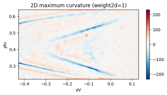
The below is the example of 2D maximum curvature

fig, ax = plt.subplots()
curvature2d(f.spectrum, dims=("phi", "eV"), alpha=0.1, weight2d=1, smooth_fn=smooth_fn).plot(ax=ax)
ax.set_title("2D maximum curvature (weight2d=1)")
fig.set_figheight(3)

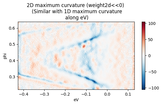
When weight2d << 0, the output is essentially same as curvature1d along eV.

fig, ax = plt.subplots()
curvature2d(f.spectrum, dims=("phi", "eV"), alpha=0.1, weight2d=-10, smooth_fn=smooth_fn).plot(
    ax=ax
)
ax.set_title("2D maximum curvature (weight2d<<0) \n (Similar with 1D maximum curvature\n along eV)")
fig.set_figheight(3)

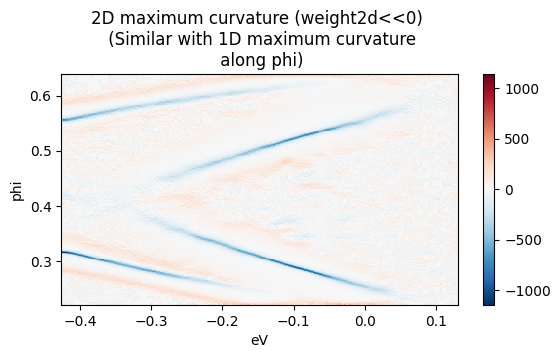
And when weight2d >> 0, the output is essentially same as curvature1d along phi.

fig, ax = plt.subplots()
curvature2d(f.spectrum, dims=("phi", "eV"), alpha=0.1, weight2d=10, smooth_fn=smooth_fn).plot(ax=ax)

ax.set_title(
    "2D maximum curvature (weight2d<<0) \n (Similar with 1D maximum curvature\n along phi)"
)
fig.set_figheight(3)

Exercises

1. Perform the following:

from  arpes.plotting import DifferentiateApp, SmoothingApp
app = DifferentiateApp(data)
app.panel()
...

derivative_result = app.output  #  Derivative, curvature, or minimum gradient result.

and then check the how the variables affect the results.